No retrocausality in QM, delayed choice quantum eraser
Luboš Motl, October 12, 2016
The delayed choice quantum eraser is a convoluted but straightforward experiment testing the quantum entanglement.

This particular experiment is usually being hyped because of the claims that it «proves» that there’s retrocausality in Nature: decisions made at a later moment may affect observations at earlier moments. In this particular experiment, these people like to say that a decision was made later – when the later member of a photon pair was detected – whether a member detected earlier should contribute to an interference pattern.
This summary of the experiment is absolutely wrong, of course. There can’t be any retrocausality – decisions that influence the past – in Nature. This principle is known as the causality: the cause always precedes its effect(s). Within the special theory of relativity, this principle has to hold according to all inertial observers – because relativity demands that all laws and principles of Nature (and causality is one of them) hold equally in all inertial systems.
One may easily see that this «causality according to all frames» implies locality. The cause not only precedes the effect, \(t_{\rm cause}\lt t_{\rm effect}\), but they must be separated by a timelike (or null) interval, too. In other words, no influence can ever propagate faster than light. This is an absolutely valid law of Nature – at least when quantum gravitational effects like black hole evaporation are banned in the discussion – and it must hold and does hold within quantum mechanics, too.
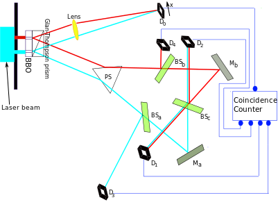
OK, what is the delayed choice quantum eraser experiment? The scheme at the top looks convoluted because it is convoluted. And people’s brains are naturally limited and when they manage to fully understand the behavior of the photons in such an experiment, they want to get something out of it. So they are more likely to buy nonsensical claims about retrocausality etc.
However, the reasons why no retrocausality exists in this experiment are very simple and universal. They apply in this experiment as well as any other experiment you may perform or just imagine. And the actual mistake that leads the people to say that some retrocausality is present are very simple-minded. To understand why these people are absolutely wrong should be easier for you than to understand the complicated geometry of this particular experiment.
The Wikipedia article makes it obvious that there’s an ongoing edit war between the crackpots who want to claim that there’s some retrocausality and the people who haven’t lost their mind. For example, a sentence says
However, the consensus contemporary position is that retrocausality is not necessary to explain the phenomenon of delayed choice. [better source needed] [18]
OK, someone tried to reduce the silly hype that this experiment implies retrocausality. Physicists generally agree that no retrocausality is needed or follows from the experiment, he pointed out. And he also picked a paper that makes the claim. This addition was immediately attacked by a pro-retrocausality jihadist. The source is not good enough etc. Well, it’s not a stellar paper but this trivial statement shouldn’t require any papers.
However, many sentences in the same article do basically say that there’s some retrocausality. For example, we may read:
However, what makes this experiment possibly astonishing is that, unlike in the classic double-slit experiment, the choice of whether to preserve or erase the which-path information of the idler was not made until 8 ns after the position of the signal photon had already been measured by D0.
But this is just a loaded interpretation of what’s going on. It’s a sentence demagogically constructed so that you may think that it’s compatible both with the observed results of the experiment as well as the idea that some later decisions affects earlier observations. However, when you look at the sentence carefully, you must agree that it’s just wrong. At the later time (8 ns after the measurement at D0), no decision was made by anybody at all. The sentence says that there was a decision so it’s just wrong. Period. (The explanations in the rest of this blog post may serve as an alternative to the period.)
The people attempting to derive contradictions and wrong claims – such as non-locality or retrocausality (or some contradictions within quantum mechanics) – are just doing silly mistakes almost everywhere. They totally distort the meaning of the words such as a decision, a cause, an effect, and many others. They’re full of šit.
OK, I must finally remind you of some technicalities of the experiment. Here’s the diagram again.

I don’t expect you to memorize the angles of all the beams. The experiment could be arranged in many different ways. None of the details are really important. But you need to know that it’s an experiment combining the double slit experiment with an entanglement experiment. And you need to know how many observables are being measured and what the measured – and quantum mechanically predicted – probability distributions are.
OK, in the upper left corner, the experiment begins as a double slit experiment. A photon may go through the (upper) red slit (sometimes also called slit A; all the paths of the photon and its offspring that would follow from its penetrating the red slit are drawn in red) or the (lower) light blue slit (sometimes also called slit B; all the subsequent paths of the photon and its offspring compatible with the penetration of slit B are drawn in light blue or cyan, if you wish).
Fine. After the photon gets through one slit or another (or their quantum superposition), it goes to the Glan-Thompson Prism, a great gift of nonlinear optics that is capable of splitting a photon to a pair of photons that are entangled with one another.
The upper member of the entangled pair of offspring photons – whether it’s a pair emerging from the photon that came through slit A=red or B=blue or some superposition – goes to the detector D0 (upper middle) that measures the location \(x\) of the photon once it lands on the detector plane. So this detector D0 is capable of drawing some intensity graph \(I(x)\) which may include some interference pattern (several quasiperiodic waves, maxima and minima) or not.
The lower member of the entangled pair of offspring photons (this photon is called the «idler» but I don’t want to bother you with the redundant terminology of the would-be «insiders») – independently of the red-or-blue which-path information of the parent – is going down (through a regular prism, beam splitters, and mirrors) and ultimately lands in exactly one of the detectors D1, D2, D3, D4. So no continuous variable such as \(x\) is measured with this photon. Instead, only a discrete variable \(M\) describing this lower photon – whose eigenvalues i.e. possible results i.e. the spectrum is \(\{1,2,3,4\}\) – is being measured.
We’re almost finished. Once again. The parent photon goes through the double slit and then this photon gets divided to a pair of children. The location \(x\) of the upper child is measured – if you made this measurement directly with the parent, you would get the simple interference pattern. But another discrete observable \(M\) describing the lower child is measured as well.
You don’t need to see the diagram of the experiment at all to understand what kind of a prediction quantum mechanics unavoidably makes, given the facts described above. Quantum mechanics predicts the probability or probability density for every choice of \(x\) – a property of the upper child photon – and every choice of \(M\) – a property of the lower child photon. What are the probabilities mathematically? They’re the function \(P(x,M)\) of one continuous variable \(x\) and one discrete variable \(M\in \{1,2,3,4\}\) that obeys the normalization
\[ \sum_{M=1}^4 \int_0^1 dx\,P(x,M) = 1. \] Maybe I should have used the name \(\rho(x,M)\) for the function \(P(x,M)\) because it’s a density relatively to \(x\). Note that I arbitrarily chose the a priori allowed values of \(x\) – position in the detector D0 – to be between \(0\) and \(1\). At any rate, the displayed equation above says that the total probability is equal to 100 percent.
Only approximately three steps are left. We must say how much \(P(x,M)\) actually is in this experiment. We must explain why quantum mechanics makes these predictions (which the actual experiment has confirmed). And we must discuss the implications for causality.
Unfortunately, none of the illustrations on the Wikipedia page is prepared so that it could be directly interpreted as a visualization of the function \(P(x,M)\). This disappointing observation is perhaps one reason – or just a side effect showing – why so many people are thinking about the correlations in this experiment irrationally. So I had to prepare a somewhat better image but I didn’t want to start from scratch and waste lots of time. So the result is:
The horizontal axis is simply \(x\) while the vertical axis is \(M\) except that \(4\) is at the bottom and… \(1\) is at the top. Because the variable \(M\) is discrete, from the set \(\{1,2,3,4\}\), the information stored in the function \(P(x,M)\) is equivalent to four functions \(P_M(x)\) of a continuous variable \(x\). And these four graphs are drawn on the picture, OK? You could draw these four graphs as a «3D plot» instead.
We’re getting to the point «why the predictions are what they are». You may notice that \(P(x,1)\) and \(P(x,2)\) show some interference pattern while \(P(x,3)\) and \(P(x,4)\) don’t. Also, the interference-free graphs of \(P(x,3)\) and \(P(x,4)\) are basically the same. On the other hand, the interference graphs \(P(x,1)\) and \(P(x,2)\) differ from each other. The former has the minima at the places of the maxima of the latter and vice versa. The sum \(P(x,1)+P(x,2)\) would look like an interference-free graph \(2P(x,3)\), too.
OK, why do two of these graphs show the interference pattern and two of them don’t?
It’s because the individual runs of the experiment with the lower photon showing up as \(M=3\) or \(M=4\) allow us to determine the which-slit information (A=red or B=blue) of the parent photon; while the \(M=1\) and \(M=2\) don’t allow us to do that. That’s why the functions \(P(x,3)\) and \(P(x,4)\) contain no interference – when you determine the which-slit information, there’s no interference. On the other hand, the functions \(P(x,1)\) and \(P(x,2)\) show interference patterns because the which-slit information is being erased and the probability amplitudes contributed by both slits are forced to interfere.
You must look at the diagram of the experiment to figure out why the value of \(M\) – the ID of the detector where the lower child photon is detected – has the influence on \(P(x,M)\) that I described in the previous paragraph.
Great. The final question is: Do these results imply any retrocausality, i.e. the ability of decisions done later to influence the observations done earlier? The question is «Not at all», of course. But we must first understand why the careless people may be tempted to think that there’s some retrocausality. They think so because they see the clear correlations between \(x\) and \(M\) encoded in \(P(x,M)\) and they can’t resist and interpret the measurement of \(M\in\{1,2,3,4\}\) as the «cause». Once we know \(M\), the wave function «collapses» and we get one of the four functions \(P_M(x)=P(x,M)\).
But it’s the discreteness of the observable \(M\) that makes the people think that \(M\) must be a «cause» of something or even the numerical ID of someone’s «decision». However, this interpretation of \(M\) is absolutely wrong. No one except for Nature’s «random generator» can decide whether \(M=1\) or \(M=2\) or \(M=3\) or \(M=4\) for a given lower photon. These four possible results have nonzero (basically equal) probabilities (25% each) and it’s up to Nature to decide which of them will become the reality for a given photon. This result is not a function of any variables in an experimenter’s brain, so the experimenter is simply not deciding about the value of \(M\).
That’s why all the statements that the measurement of \(M\) – the information in which detector D1, D2, D3, D4 the lower photon emerges – are «decisions» are absolutely wrong. No human or other decision can influence the result which is up to Nature’s «random generator».
But not only the statement that the value of \(M\) is a «decision» is absolutely wrong. The statement that it is a «cause» of anything is wrong, too. The people who say that \(M\) is a «cause» responsible for the detailed correlation between \(x\) and \(M\) – the detailed form of the function \(P(x,M)\) – are imagining that discrete observables must be «primary». They may imagine an «engine» which takes some discrete input such as \(M\in\{1,2,3,4\}\) and produces an output, either the function \(P_M(x) = P(x,M)\) or the random number \(x\) chosen from that distribution \(P(x,M)\). And they think that it can’t be the other way around. That’s why, they think, \(M\) must be an «input» of a «program» while \(x\) is a random «output» of the «program», chosen by a random generator according to the probability distribution \(P_M(x) = P(x,M)\).
These people can’t imagine that it’s the other way around, that \(x\) is an «input» and \(M\) is an «output». So they just can’t imagine that the «collapse» induced by the measurement of \(x\) of the upper photon is the «cause» that affects the probabilities for the value of \(M\) measured later. However, this prejudice that the discrete observables must be the «input» while continuous ones must only be an «output» is absolutely irrational.
When it comes to the causality issues, there’s no qualitative difference between discrete and continuous variables.
OK, the wrong people are capable of imagining that one first collapses the full distribution (or the wave function from which it is calculated) to the part \(M=2\) and the complex distribution \(P(x,M)\) gets replaced by the simpler \(P(x,2)\), for example. (Well, we need to normalize it, so \(P(x,2)\) in the previous sentence should be replaced with the conditional probability \(P(x,2)/P_2\) where \(P_2=\int_0^1 dx\,P(x,2)\to 1/4\).) But they can’t imagine that the collapse according to \(x\) occurs first.
But it is equally sensible to run the logic backwards – because the graph that I repeated above may be read or sliced both horizontally and vertically! We may measure the location of the upper photon \(x\) first. If you want a «classical simulation» of quantum Nature, the probability distribution \(P(x)\) according to which the resulting \(x\) is being randomly selected is simply
\[ P(x) = \sum_{M=1}^4 P(x,M). \] Note that
\[ \int_0^1 dx\, P(x) = 1 \] because of the previously written condition. Once you pick \(x\) according to this distribution, you still have to randomly decide what the \(M\) that you measure later will be. What are the probabilities \(P_M\) of different values \(M\in\{1,2,3,4\}\) given the condition that the upper child photon has been seen at the location \(x\)? Well, it’s simply the conditional probability
\[ P_M = \frac{P(x,M)}{P(x)} \] The \(M\)-independent denominator is there to guarantee the normalization condition
\[ \sum_{M=1}^4 P_M = 1. \] Note that the «division by zero» can’t occur in the formula for \(P_M\) because the denominator is \(P(x)\) which was the probability that the upper child photon lands at the point \(x\). So the probability that we have to deal with the division by zero is… zero.
To be specific, if \(x\) is first measured near the maxima of \(P(x,1)\), it will be more likely that the value of \(M\) will be measured as \(M=1\), and so on.
If you write a classical simulation which does the things in this way, you will realize that there is absolutely nothing wrong about the fact that the collapse according to the measured value of \(x\) occurs first – and in this sense, the measurement of \(x\) looks like a cause affecting the later measurement of \(M\). Even if you repeat the same experiment many times, the only thing that you may actually experimentally determine is the probabilistic distribution \(P(x,M)\). And this distribution is given by a graph of «two variables» and it doesn’t matter a single bit whether you slice this function of two variables horizontally or vertically!
In other words, it’s absolutely inconsequential whether the measurement of \(x\) was done before the measurement of \(M\) or vice versa. The whole function \(P(x,M)\) determining all probabilities and correlations was determined before either of the two measurements took place. This statement means that no event that took place later could have changed anything about the odds. So there was simply no cause after the initial transmission through the double split; and after the splitting of the photon by the prism.
The classical simulations which produced the random results according to the distributions needed to remember when some distributions should be collapsed etc. But all these choices were mere artifacts of the classical computer simulation. The physically meaningful information about all the possible results of the experiment is fully encoded in the function \(P(x,M)\). Once \(P(x,M)\) is determined, and it’s determined very early on, all the actual «causes» (events that influence others) have already taken place and the predictions are clear. No new causes, influences, impact, or communication takes place afterwards.
To slice \(P(x,M)\) into four functions \(P_M(x)\) or infinitely many discrete distributions \(P_M^{\to x}\) are just different ways to think about exactly the same reality, exactly the same odds. They don’t physically differ at all. So once again, the actual causes explaining all the correlations – the presence or absence of an interference pattern in \(P_M(x)\) depending on \(M\) – are events that take place at the very beginning of the experiment.
However, we may simplify our life by making «collapses» of the data – replacing the most general wave function or probability distribution \(P(x,M)\) with the conditional probabilities or probability distributions where the already measured data are assumed to be facts. When we do so, the ordering of the collapses may be arbitrary. \(x\) may collapse before \(M\) or vice versa. It always works the same.
The idea that the correlation (\(M\)-dependence of the presence of the interference pattern in \(P_M(x)\)) requires some non-local action at the moment of the measurement is wrong. But the idea that this action must be ordered so that the collapse of \(M\) is a «cause» and the (earlier) collapse into some point \(x\) is an «effect» – is even more wrong. The latter silly viewpoint – the idea that this experiment implies some retrocausality – is nothing else than some people’s inability to slice graphs of \(P(x,M)\) both vertically and horizontally. It’s absolutely stupid.
This two-month-old PBS Spacetime video with 570,000 views and almost 99% of positive votes has led me to write this blog post. And it is another example of a source where almost every big claim is completely wrong and stupid. While it is absolutely stupid, these delusions are the very reason why certain people spend so much time with these convoluted experiments. The experimenters clearly want to deceive the readers and many of the readers clearly want to be deceived.
But if you think rationally about the text above and a few other blog posts, you may easily understand the full logic of quantum mechanics and the causal influences in it. The results of entanglement don’t require and don’t prove any communication at the moment of the measurement. There’s never any retrocausality in Nature. If commutators of spacelike-separated fields vanish (like in quantum field theory), the choice «what to measure» doesn’t affect any predictions for faraway (spacelike-separated) observations which is why there’s no action at a distance (but when you actually know the results of your experiment, it does affect your expectations of the faraway results if there are correlations – and correlations are almost always there iff the two subsystems have interacted or been in contact in the past).
When your brain approaches all these issues sensibly, your knowledge won’t be vulnerable to another, more complex or more confusing experiment. What I write about quantum mechanics is absolutely valid. No experiment, however convoluted, can be exempted. Quantum mechanics demands that you abandon realism – the idea that things have objectively unique and well-defined properties even without or prior to the observations. But no other «common sense» principle – such as locality and causality – is being rejected by quantum mechanics.


