On the importance of conformal field theories

Luboš Motl, June 30, 2012

Scale-invariant theories may look like a too special, measure-zero subset of all quantum field theories. But in the scheme of the world, they play a very important role which is why you should dedicate more than a measure-zero fraction of your thinking life to them.

In this text, I will review some of their basic properties, virtues, and applications.

When we look at Nature naively and superficially, its laws look scale-invariant. One may study a hamburger of a given weight. However, it seems that you may also triple the hamburger’s weight and the physical phenomena will be mathematically isomorphic. Just some quantities have to be tripled.

(Sean Carroll has tried to revive the old idea of David Gross to sell particles to corporations in order to get funding for science; search for David Rockefeller quark in that paper. The Higgs boson could be sold to McDonald’s, yielding a McDonald’s boson. However, anti-corporate activist Sean Carroll has failed to notice that McDonald’s actually deserves to own the particle for free because much like the God particle, McDonald’s is what gives its consumers their mass.)

The scale invariance seems to work

For example, if you triple the radii of all planets, the masses will increase 27-fold if you keep the density fixed. To keep the apparent sizes constant, you must also triple the distances. The forces between these planets will increase by the factor of \(27\times 27 / 3^2 = 81\), accelerations by the factor of \(27/3^2=3\). If you realize that the centrifugal acceleration is \(r\omega^2\) and \(r\) was tripled, you may actually get the same angular frequency \(\omega\).

With different assumptions than a constant density and the prevailing gravitational force, you might be forced to scale \(\omega\) and times in a different way, and so forth.

But it’s broken

However, when you look at the world more carefully and you uncover its microscopic and fundamental building blocks, and maybe even earlier than that, you will notice that no such scale invariance actually exists. A 27-times-heavier planet contains 27-times-more atoms; this integer is different so the two planets are definitely not mathematically isomorphic.

And atoms can’t be expanded. Atoms of a given kind always have the same mass. They have the same radius (in the ground state). As the Universe expands, the atoms’ size remains the same so the number of atoms that may «fit» into some region between galaxies is genuinely increasing. The atoms emit spectral lines with the same frequency and wavelength. After all, that’s why we may define one second as the duration of 9,192,631,770 periods of the radiation corresponding to the transition between the two hyperfine levels of the ground state of the caesium 133 atom. Even well-behaved tiny animated GIFs blink once in a second and no healthy computer should ever change the frequency. 😉

And even the Gulliver is a myth. More precisely, and the experts in literature could correct me, the Gulliver is a normal man but the Lilliputians are a myth. 😉 You can’t just scale the size of organisms. Such a change of the size has consequences. Too small or too large copies of a mammal would have too weak bones to support the body, they would face too strong a resistance of the air, they couldn’t effectively preserve their body temperature different from the environment’s temperature, and so on, and so on.

The period of some atomic radiation is constant and may be measured very accurately which is why it’s a convenient benchmark powering the atomic clocks – the cornerstone of our definition of a unit of time. However, it’s not necessarily the most fundamental quantity with the units of time. In particle physics, the de Broglie wave associated with an important particle at rest yields a «somewhat» more fundamental frequency than the caesium atom. In quantum gravity, the Planck time may be the most natural unit of time.

Scale invariance in classical and quantum field theories

How do we find out that some laws of physics are scale–invariant? Well, there won’t be any preferred length scale in the phenomena predicted by a theory if the fundamental equations won’t have a preferred length scale. They must be free of explicit finite parameters with units of length; but they must also be free of parameters whose powers could be multiplied to obtain a finite result with the units of length.

For example, the Lagrangian density of Maxwell’s electromagnetism is\[

{ \mathcal{L}_{Maxwell}} = -\frac 14 F_{\mu\nu}F^{\mu\nu}.

\] The sign is determined by some physical constraints: the energy must be bounded from below. The factor of \(1/4\) is a convention. It is actually more convenient than if the factor were \(1\) but the conceptual difference is really small. What’s important is that there are no dimensionful parameters. If you wrote electromagnetism with such parameters, e.g. with \(\epsilon_0\) and \(c\), you could get rid of them by a choice of units and rescaling of the fundamental fields. And whenever it’s possible to get rid of the parameters in this way, the theory is scale-invariant.

When we deal with a scale-invariant theory, it doesn’t mean that all objects are dimensionless. Quite on the contrary: most of the quantities are dimensionful. The scale invariance is actually needed if you want to be able to assign the units to quantities in a fully consistent way. When you have a theory with a characteristic length scale, i.e. a non-scale-invariant theory, you may express all distances in the units of the fundamental length unit (e.g. Planck length). All distances effectively become dimensionless and the dimensional analysis tells you nothing.

However, in a scale-invariant theory, you may assign the lengths and spatial coordinates the units of length, e.g. one meter. The partial derivatives \(\partial/\partial x\) will have the units of the inverse length. Because \(S\) must be dimensionless in a quantum theory – \(iS\) appears in the exponent in Feynman’s path integral – it follows that the Lagrangian density has to have units of \({\rm length}^{-4}\). That’s because \(S=\int{d^4 x  \mathcal{L}}\). I have implicitly switched to a quantum field theory now and set \(\hbar=c=1\) which still prevents us from making lengths or times (or, inversely, momenta and energy) dimensionless.

In the electromagnetic case, the units of \( \mathcal{L}\) are \({\rm length}^{-4}={\rm mass}^4\) which means that \(F_{\mu\nu}=\partial_\mu A_\nu-\partial_\nu A_\mu\) has to have the units of \({\rm mass}^2\). And because \(\partial_\mu\) has the units of \({\rm mass}\) i.e. \({\rm length}^{-1}\), we see that the same thing holds for \(A_\mu\). In this way, all degrees of freedom may be assigned unambiguous units of \({\rm mass}^\Delta\) where \(\Delta\) is the so-called dimension of the degree of freedom (a particularly widespread concept for quantum fields).

In classical field theory, the dimensions would always be rational – most typically, \(\Delta\) would be integer or, slightly less often, a half-integer. However, in quantum field theory, the dimension of operators often likes to be an irrational number. Whenever perturbation theory around a classical limit works, these irrational numbers may be written as the classical dimensions plus «quantum corrections to the dimension», also known as the anomalous dimensions. The leading contributions to such anomalous dimensions in QED are often proportional to the fine-structure constant, \(\alpha\approx 1/137.036\). This correction to the dimension may be calculated from some appropriate Feynman diagrams.

At any rate, all fields – including composite fields – may be assigned some well-defined dimensions \(\Delta\). If distances triple, the fields must be rescaled by \(3^{-\Delta}\).

Now, how many scale-invariant theories are there? Do we know some of them? Well, among the renormalizable theories such as the Standard Model, there is always a «natural» cousin or starting point, a quantum field theory that is classically scale-invariant. The actual full-fledged theory with mass scales is obtained by adding some mass terms and similar terms to the Lagrangian. It’s easy to be explicit what we mean. The classically scale-invariant theory is simply obtained by keeping the kinetic terms – the terms with the derivatives – only and erasing the mass terms as well as all other terms with coefficients with units of a positive power of length.

It means that to get a scale-invariant theory, you keep \(F_{\mu\nu}F^{\mu\nu}\), \(\partial_\mu \phi\cdot \partial^\mu\phi\), \(\bar\psi\gamma^\mu \partial_\mu \psi\) etc. but you erase all other terms, especially \(m^2 A_\mu A^\mu\), \(m^2\phi^2\), \(m\bar\psi\psi\), and so on. Is there a justification why we can neglect those terms? Yes. We’re effectively sending \(m\to 0\) i.e. we’re assuming that \(m\) is negligible. Can \(m\) be negligible? It depends whom you compare it with. It’s negligible relatively to much greater masses/energies. That’s why the mass terms and similar terms may be neglected (when we study processes) at very high energies i.e. very short distances. That’s where the kinetic terms are much more important than the mass terms.

I said that by omitting the mass terms, we only get «classically» scale-invariant theories. What does «classically» mean here? Well, such theories aren’t necessarily scale-invariant at the quantum level. The mechanism that breaks the scale invariance of classically invariant theories is known as the dimensional transmutation. It has a similar origin as the anomalous dimensions mentioned above. Roughly speaking, the Lagrangian density of QCD, \(-{\rm Tr}(F_{\mu\nu} F^{\mu\nu})/2g^2\), no longer has the units of \({\rm mass}^4\) but slightly different units, so a dimensionful parameter \(M^{\delta\Delta}\) balancing the anomalous dimension has to be added in front of it. In this way, the previously dimensionless coefficient \(1/2g^2\) that defined mathematically inequivalent theories is transformed into a dimensionful parameter \(M\) – which is the QCD scale in the QCD case – and the rescaling of the coefficient may be emulated by a change of the energy scale. So different values of the coefficient are mathematically equivalent after the dimensional transmutation because the modified physics may be «undone» by a change of the energy scale of the processes.

Ability of fixed points to be unique up to a few parameters

In the previous paragraphs I discussed a method to obtain a scale-invariant quantum field theory by erasing all the mass terms in an arbitrary quantum field theory. This procedure is actually more fundamental than how it may look. The scale-invariant theory is a legitimate fundamental starting point to obtain almost any important quantum field theory we know.

The reason is that the ultimate short-distance limit of a generic consistent quantum field theory has to be scale-invariant. When we study energies higher than all typical energy scales in a quantum field theory, all these energy scales associated with the given scale-non-invariant theory may be neglected and we’re bound to get a scale-invariant theory in the limit. Such a limiting short-distance theory is known as the UV fixed point. The adjective UV, or ultraviolet, means that we talk about short-distance physics. The term «fixed point» means that it is a scale-invariant theory: it is invariant (fixed) under the scaling of the distances (deriving longer-distance physics from short-distance physics) which is the basic operation we do in the so-called Renormalization Group, a modern framework to classify quantum field theories and their deviations from scale invariance in particular.

A funny thing is that scale-invariant theories are very restricted. For example, the \( \mathcal{N}=4\) gauge theory is unique for a chosen gauge group (up to the coupling constant and the \(\theta\)-angle). Its six-dimensional ancestor, the (2,0) superconformal field theory, is also scale-invariant and it is completely unique for chosen discrete data.

In other cases, the space of possible scale-invariant field theories is described by a small number of parameters. Even when we study the deformations of these theories that don’t break the renormalizability, we only add a relatively small number of parameters. The condition that an arbitrary quantum field theory is renormalizable (and consistent up to arbitrarily high energy scales) is pretty much equivalent to the claim that one may derive its ultimate short-distance limit which is a UV fixed point.

It’s this existence of the scale-invariant short-distance limit that makes our quantum field theories such as the Standard Model predictive. We may prove that there’s only a finite number of parameters that don’t spoil the renormalizability i.e. the ability to extrapolate the theory up to arbitrarily short distances. And when we extrapolate the theory to vanishingly short distances, we inevitably obtain one of the rare scale-invariant theories which only depend on a small number of parameters (and some discrete data).

So the scale-invariant theories aren’t just an interesting subclass of quantum field theories that differs from the rest; for each consistent scale-non-invariant quantum field theory, there exists an important scale-invariant theory, namely the short-distance limit of it. There is another scale-invariant theory for each quantum field theory, namely its ultimate long-distance limit. Both of these limits may be – and often are – non-interacting theories because the coupling constants of QCD-like theories may slowly diminish. Also, the long-distance limit, the infrared fixed point, is often a theory with no degrees of freedom: it is «empty». For example, QCD predicts the so-called «mass gap» – the claim that all of its particles that may exist in isolation have a finite mass (the mass can’t be made zero or arbitrarily small). So if you only study particle modes that survive below a certain very low energy, you get none.

No doubts about that: scale-invariant theories are very important for a proper understanding of all quantum field theories. They also play a key role in string theory, at least for two very different reasons – perturbative string theory and the AdS/CFT correspondence. These roles will be discussed in the rest of this blog entry.

Scale-invariant vs conformal

Before I jump on these stringy issues, let me spend a few minutes with a subtle difference between two adjectives, «scale-invariant» and «conformal». A scale-invariant theory is one that has the following virtue: for every allowed object, process, or history (one that obeys the equations of motion or one that is sufficiently likely according to some probabilistic rules), it also allows objects, processes, and history that differ from the original one by a scaling (or these processes are equally likely).

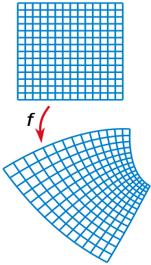
A conformal i.e. angle-preserving map. In two Euclidean dimensions, it’s equivalently a (locally) holomorphic function of a complex variable. Note that all the intersections have 90-degree internal angles.

The adjective «conformal» is a priori more constraining: for a given objects, processes, and histories, a conformal theory must also guarantee that all processes, objects, and histories that differ from the original one by any (possibly nonlinear) transformation of space(time) that preserves the angles (between lines, measured locally) – any conformal map – must also be allowed. Conformality is a stronger condition because scaling is one of the transformations that clearly preserve angles but there are many more transformations like that.

While conformality is a priori a stronger condition than scale invariance, it turns out – and one can prove – that given some very mild additional assumptions, every scale invariant theory is automatically conformally invariant. I won’t be proving it here but it’s intuitively plausible if you look what the theory implies for small regions of spacetime. In a small region of spacetime (e.g. in the small squares in the picture above), every conformal transformation reduces to a composition of a rotation (or Lorentz transformation) and a scaling. So if these transformations are symmetries of the theory and if the theory is local, it must also allow you to perform transformations that look «locally allowed» (locally, they are rotations combined with scaling) – it must allow conformal symmetries.

Now, what is the group of conformal transformations in a \(d\)-dimensional space? Start with the Euclidean one. The group of rotations is \(SO(d)\). What about the conformal group, the group of transformations preserving the angles? One may show that transformations such as \(r\to 1/r\), the inversion, preserve the angles. A conceptual way to see the whole group is the stereographic projection:

You may identify points in a \(d\)-dimensional flat space with points on a \(d\)-dimensional sphere – the boundary of a \((d+1)\)-dimensional ball – by the stereographic projection above. A funny thing you may easily prove is that this map preserves the angles. For example, if you project the Earth’s surface from the North Pole to the plane tangent to the South Pole, you will get a map of the continents that will locally preserve all the angles (but not the areas!).

It follows that all the isometries of the sphere, \(SO(d+1)\), must generate some conformal maps of the plane. In fact, one may do the same thing with a projection of the plane from a hyperboloid or Lobachevsky plane – the sphere continued to a different signature. For this reason, the conformal group must contain both \(SO(d+1)\) and \(SO(d,1)\) as subgroups: it must be at least \(SO(d+1,1)\). One may show that there are no other transformations,too.

To get the conformal group, you write the rotational group as \(SO(m,n)\) and add one to each of the two numbers to get \(SO(m+1,n+1)\). Because the Minkowski space is a continuation of the sphere, a continuation of the procedures above proves that the same thing holds for the conformal group of a \(d\)-dimensional spacetime. While the Lorentz group is \(SO(d-1,1)\), the conformal group is \(SO(d,2)\). Yes, it has two time dimensions. This group \(SO(d,2)\) contains not only the Lorentz group but also the translations, scaling, and some extra transformations known as the special conformal transformations.

Role of conformal field theories in AdS/CFT

The group \(SO(d,2)\) is the conformal group of a \(d\)-dimensional Minkowski space. However, it’s also the Lorentz symmetry of a \(d+2\)-dimensional spacetime with two timelike dimensions. In fact, we don’t need the whole \((d+2)\)-dimensional spacetime. It’s enough to consider all of its points with a fixed value of

\[x_\mu x^\mu = \pm R^2,\quad x^\mu \in \mathbb{R}^{d+2}\]

For a properly chosen sign on the right hand side (correlated with the convention for your signature), this is a «hyperboloid» with the signature of the induced metric that has \(d\) spatial dimensions and \(1\) time dimension. This hyperboloids is nothing else than the anti de Sitter (AdS) space, namely the \((d+1)\)-dimensional one.

So for every conformal transformation on the \(d\)-dimensional flat space, there is an isometry of the \(AdS_{d+1}\) anti de Sitter space. If we start with a conformal theory in \(d\) dimensions, there could also be a theory on \(AdS_{d+1}\) that is invariant under the isometries of this anti de Sitter space. Juan Maldacena was famously able to realize this thing – during his research of thermodynamics of black holes and black branes in string theory – and find strong evidence in favor of his correspondence.

For every (non-gravitational, renormalizable, healthy) conformal (quantum) field theory in a flat space, there exists a consistent quantum gravitational (and therefore non-scale-invariant) theory (i.e. a vacuum of string/M-theory) living in a curved spacetime with one extra dimension, the \((d+1)\)-dimensional anti de Sitter space, and vice versa. I was predecided to keep this section short. Although the AdS/CFT is arguably the most important development in theoretical physics of the last 15 years, it’s been dedicated enough space and I realize that if I started to explain various aspects of this map, we could easily end up with a document that has 261 pages much like the AdS/CFT Bible by OGOMA, not to be confused with the author of a footnote in a paper about the curvature of the constitutional space. His name was OBAMA. 😉

The AdS/CFT correspondence is important because it makes the holography in quantum gravity manifest, at least for the AdS spacetimes. Also, it allows us to define previously vague and mysterious theories of quantum gravity in terms of seemingly less mysterious non-gravitational (and conformal) quantum field theories. Well, it also allows us to study complex phenomena in hot environments predicted by conformal field theories in terms of more penetrable – and essentially classical – general relativity in a higher-dimensional space. Complex phenomena including low-energy physics heroes such as the quark-gluon plasma, superconductors, Fermi liquids, non-Fermi liquids, and Navier-Stokes fluids may be studied in terms of simple black holes in a higher-dimensional curved spacetime.

Role of 2D conformal field theories in perturbative string theory

Because of the chronology of the history of physics, it would have been logical to discuss the role of conformal field theories in perturbative string theory before the AdS/CFT. I chose the ordering I chose because the AdS/CFT is closer to the «more field-theoretical» aspects of string theory than the world sheet CFTs underlying perturbative string theory – something that is as intrinsically stringy as you can get. That’s why the discussion of two-dimensional CFTs was finally localized in the last section of this blog entry.

The textbooks of string theory typically tell you that strings generalize point-like particles. While point-like particles have one-dimensional world lines in the spacetime, strings analogously leave two-dimensional world sheets as the histories of their motion in spacetime.

If you want point-like particles to interact with each other, you need «vertices» of Feynman diagrams; you need points on the world lines from where more than two external world lines depart. Such a vertex is a singular point and this singularity on the world lines – the vertices in the Feynman diagrams themselves – are the ultimate cause of the violent short-distance behavior of point-like-particle-based quantum field theories, especially if there are too many vertices in a diagram and if they have too many external lines.

An idea to defeat this sick short-distance behavior is to have higher-dimensional extended elementary building blocks. In that case, you may construct «smooth versions» of the Feynman diagrams on the left – but the «smooth versions» have the property that they’re locally made of the same smooth higher-dimensional surface. The pants diagram on the right side of the picture – the two-dimensional world sheet depicted by this illustration – has no singular points.

However, there’s a catch: if the fundamental building blocks have more than 2 spatial dimensions, the internal theory describing the world volume themselves is a higher-dimensional theory and to describe interesting interacting higher-dimensional theories like that, you will need «something like quantum field theory» which will have a potentially pathological behavior that is analogous to the behavior of quantum field theories in ordinary higher-dimensional spacetimes.

Two dimensions of the world sheet is the unique compromise for which you may tame the short-distance behavior in the spacetime – because you don’t need «singular» Feynman vertices and the histories are made of the same «smooth world sheet» everywhere; but the world sheet theory itself is under control, too, because it has a low enough dimension.

In fact, an even more accurate explanation of the uniqueness of two-dimensional world sheets is that you may get rid of the world volume gravity in that case. Imagine that you embed your higher-dimensional object into a spacetime by specifying coordinates \(X^\mu(\xi^i)\) where \(\xi^i\) [pronounce: «xi»] are \(d\) coordinates parameterizing the world line, world sheet, or world volume. With such functions, you may always calculate the induced metric on the world volume

\[h_{ij} = g_{\mu\nu} \partial_i X^\mu \partial_j X^\nu\]

If you also calculate

\[ds^2 = h_{ij} d\xi^i d\xi^j\]

using the induced metric \(h_{ij}\) for some small interval on the world sheet \(d\xi^i\), you will get the same result as if you calculate it using the original spacetime metric \(g_{\mu\nu}\) with the corresponding changes of the coordinates \(dX^\mu = \partial_i X^\mu\cdot d\xi^i\). It’s kind of a trivial statement; you may either add the partial derivatives while calculating \(dX^\mu\) from \(d\xi^i\) or while calculating \(h_{ij}\) from \(g_{\mu\nu}\).

So even if you decide that the induced metric isn’t a «fundamental degree of freedom» on the world volume, it’s still there and if the shape of the string or brane is dynamical, this induced metric field is dynamical, too. You deal with a theory that has a dynamical geometry – in this sense, it is a theory of gravity. However, something really cool happens for two-dimensional world sheets: you may always reparametrize \(\xi^i\) by a change of the world sheet coordinates – given by two functions \(\xi^{\prime i} (\xi^j)\) – and bring the induced metric to the form

\[h_{ij} = e^{2\varphi(\xi^k)} \delta_{ij}\]

where \(\delta\) is the flat Euclidean metric; you may use \(\eta_{ij}\) in the case of the Minkowski signature, too. So up to a local rescaling, the metric is flat! It’s easy to see why you can do such a thing. The two-dimensional metric tensor only has three independent components, \(h_{11},h_{12},h_{22}\) and the diffeomorphism depends on two functions so it allows you to remove two of the three components of the metric. The remaining one may be written as a scalar multiplying a chosen (predecided) metric such as the flat one. At least locally, i.e. for neighborhoods that are topologically disks, it is possible.

And if the world sheet theory is conformally invariant, it doesn’t depend on the local rescaling. It doesn’t depend on \(\varphi\), either. So every world sheet is conformally flat which means that as far as physics goes, it’s flat! At least locally. There are obviously no problems with the quantization of gravity if the «spacetime», in this case the world sheet, is flat.

Many things simplify. For example, the Nambu-Goto action, generalizing the length of the world line of a point-like particle, is the proper area of the world sheet which is an integral of the square root of the determinant of the induced metric. This looks horribly non-polynomial etc. You may be scared of the idea to develop Feynman rules for such a theory. However, if you exploit the possibility to choose an auxiliary metric and make it flat by an appropriate diffeomorphism, the action actually reduces to a kindergarten quadratic Klein-Gordon action for the scalars \(X^\mu(\xi^i)\) propagating on the two-dimensional world sheet!

That’s really cool because the resulting modes of the string inevitably contain things like the graviton polarizations in the spacetime. So you may describe gravity in terms of things that are as simple and as controllable as free Klein-Gordon fields in a different space, the two-dimensional world sheet.

I said that the conformal symmetry for a \(d\)-dimensional space is \(SO(d+1,1)\) and/or \(SO(d,2)\), depending on the signature. But in two dimensions, this group is actually enhaced to something larger: the group of all angle-preserving transformations is actually infinite-dimensional (as long as you don’t care whether the map is one-to-one globally and you only demand that it acts nicely on an open set of the disk topology). In the Euclidean signature, they’re nothing else than all the holomorphic functions of a complex variable; in the case of the Lorentzian signature, one may redefine \(\xi^+\) to any function of it and similarly for \(\xi^-\), the other lightlike coordinate. The variables \(\xi^\pm\) are the continuations of \(z,\bar z\), the complex variable and its conjugate. It’s not shocking that we may redefine the lightlike coordinates by any functions and independently: the angles in a two-dimensional Minkowski space are given as soon as you announce what the two null directions are; but the scaling of each of them is inconsequential for the (Lorentzian) angles i.e. rapidities.

The conformal symmetry plays an important role for the consistency and finiteness of string theory, at least in the (manifestly Lorentz-)covariant description of perturbative string theory. States of a single string are uniquely mapped to local operators on the world sheet (that’s true even for higher-dimensional CFTs); the OPEs (operator product expansions) encode the couplings between triplets of string states; the loop diagrams are obtained as integrals over the possible shapes of the world sheet of a given topology (genus) and these shapes reduce to finite-dimensional conformal equivalence classes. So all the loop diagrams may be expressed as finite-dimensional integrals over manifolds – spaces of possible shapes of the world sheet – which are under control.

Again, this article doesn’t want to go too deeply to either of these topics because I don’t want to reproduce Joe Polchinski’s book on string theory here. Instead, this blog entry was meant to provide you with a big-picture framework answering the question «Why do the conformal field theories get so much attention?».

I feel that this kind of questions is often asked and there aren’t too many answers to such questions in the standard education process etc.

And that’s why I wrote this memo.