Why are there spinors?
Luboš Motl, April 26, 2012
Spinors are competitors of vectors and tensors. In other words, they are representations of the orthogonal (rotational) group or the pseudoorthogonal (Lorentz) group, a space of possible objects whose defining property is the very characteristic behavior of their components under these transformations.
Spinors are important to describe any particle with the spin equal to \(j=1/2\), the smallest allowed positive amount of the intrinsic angular momentum. Because they describe the wave functions (and, correspondingly, the quantum fields) associated with electrons, neutrinos, other leptons, quarks, and perhaps other particles, they’re a part of the vital mathematical toolkit servicing the well-established portion of physics.
They are also key players in concepts of cutting-edge and speculative physics including supersymmetry; and the most complicated and least understood ones among the simple representations of the orthogonal groups.
Vectors and tensors
Spinors hide a similar idea as tensors but they are not tensors. Nevertheless, it is a good idea to start with tensors.
Consider a three-dimensional Euclidean space, for the sake of concreteness. It is made out of vectors
\[\vec V = (V_x,V_y,V_z)\]
These three coordinates apply to a specific basis, a particular choice of the coordinate axes. What happens if we rotate these axes? The coordinates change. They will change to some combinations
\[\vec V\to \vec V’ = M\cdot \vec V, \qquad V_m = \sum_{n=1}^3 M_{mn} V_n\]
The symbol \(\sum_n\) for the summation over the doubly repeated index \(m=x,y,z\) may be omitted and will be omitted. If an index appears twice, you always imagine that there is a sum over all of its possible values in front of the expression. We call this modified rule of mathematics the Einstein summation rule.
The matrix \(M\) is composed of the entries \(M_{mn}\) where the convention says that the first index \(m\) describes which row the entry is written at; \(n\) tells us which column we look at. If we expect the length of all vectors such as
\[L(\vec V) = \sqrt{V_x^2+V_y^2+V_z^2}, \qquad L(\vec V’)=L(\vec V)\]
to be preserved, we need to allow orthogonal transformations only. They have to obey
\[M\cdot M^T ={\bf 1}\]
Note that the equation above says that \(M\) and the transposed matrix (recall that \(M^T_{mn}\equiv M_{nm}\)) \(M^T\) are inverse to each other, so it automatically follows that
\[M^T\cdot M ={\bf 1}\]
holds as well. The left inverse is automatically the right inverse and vice versa. Matrices obeying this rule are known as orthogonal matrices (encoding the corresponding orthogonal transformations) and their set is known as the orthogonal group \(O(N)\). In our case, we talk about \(O(3)\). If we also demand that \(\det M=+1\) and not \(\det M=-1\) which is the other allowed value (the «mirroring» transformations), we deal with the special orthogonal group \(SO(N)\) i.e. \(SO(3)\) in our case.
However, it’s also possible to consider all invertible linear transformations, whether they preserve angles and distances or not. The group is known as \(GL(N)\), the general linear group, and the subgroup with the determinant equal to one is \(SL(N)\). If we talk about all linear (or all special linear) transformations, we should distinguish upper and lower indices. If the components with the upper indices get 5 times larger, for example, the components with lower indices have to get 5 times smaller (transform according to the inverse matrix) for the expressions like \(V^m W_m\) to be preserved.
Tensors: now really
While many important quantities – position, velocity, momentum, electric field strength etc. – transform as vectors, there are also other important «collections of components» that may transform if you change your coordinate system. And I don’t mean just pseudovectors – angular momentum, magnetic field strength etc. – which transform just like vectors under \(SO(N)\) but pick the opposite sign under the transformations from the other part of \(O(N)\). Instead, I am talking about objects that transform differently even under \(SO(N)\), the tensors.
Pragmatically speaking, a tensor is a collection of components
\[T = \{ T_{mnop\dots z} \}\]
with many indices. To make my first tensor impressive, I’ve included one-half of the Latin alphabet or so. However, aside from the «scalars» which have no indices and «vectors» which have one index and have already been discussed, the simplest new tensors have two indices. Much like the components of the vector \(\vec V\) transformed to those of \(\vec V’\) under the transformation given by \(M\), a matrix, the same is true for tensors whose transformation rule is
\[{\bf T}\to {\bf T’} , \qquad T_{mp} = M_{mn} M_{pq} T_{nq}\]
We have used the Einstein summation rule. Note that aside from \(M_{mn}\) which is attached to the index \(n\) in \(T_{nq}\) and the index \(n\) is summed over, the final expression also contains an analogous factor \(M_{pq}\) which is attached to the new summed-over index \(q\) in \(T_{nq}\). For every index in the tensor, you include one factor of the matrix into the transformation rule. The doubly repeated indices are summed over.
You may see that the rule for the transformation of \(T\) is exactly the same as if \(T\) were a tensor product of two vectors \(\vec V,\vec W\),
\[T_{mp} = V_m W_p\]
If you studied how the \(N\times N\) components which are products of the components of vectors transform, you would get exactly the same rule. So the tensors transform just like tensor products of vectors. (Tensor products mean that we’re not summing over any indices, like we are in the inner products, and we’re not even adding any epsilon to sum over, like in cross products: we just keep all the products of components to produce a more extensive collection of components.)
That doesn’t mean that every tensor is a tensor product of two (or a higher number of) vectors. For example, in three dimensions, the general tensor with 2 indices has 9 components while two vectors only have 6 components (and one of them doesn’t matter because if you rescale one vector by a factor and reduce the other by the same factor, their tensor product won’t change). But a tensor may always be represented as a sum of such tensor products of vectors.
The advantage of tensors is that whenever we construct any other tensor out of tensor products of some input tensors, or contractions of them (summation over repeated indices which reduces the total number of indices of a tensor, like the inner product is a contraction of the tensor product of two vectors \(T_{mm}=V_m W_m\)), these contracted or uncontracted products still transform according to the general rule for tensors. In particular, if you manage to construct a scalar as a contraction of a tensor (which may be a product of many tensors itself), this scalar will have the same value in all coordinate systems.
Tensors are useful to define quantities such as the moment of inertia \(I_{mn}\). The kinetic energy, a typical scalar, may be written as
\[E = \frac{1}{2} I_{mn} \omega_m \omega_n\]
where \(\omega\) is the vector (well, pseudovector) of angular velocity. The equation above makes it clear that only the symmetric part \((I_{mn}+I_{nm})/2\) matters so the tensor may be assumed to be symmetric. It’s one of the many mathematical facts that by making a rotation, a symmetric tensor may be brought into a diagonal form so that \(I_{mn}\) is nonzero only if \(m=n\). The diagonal entries \(I_{mm}\) (no summation here, exception) describe the moment of inertia for rotations around the three privileged axes.
All this tensor calculus may be generalized to any spacetime dimension, any signature. The tensors may have any number of indices. We may use tensors for the most general linear transformations from \(GL(N,\mathbb{R})\) or even \(GL(N,\mathbb{C})\). In that case, however, we must carefully distinguish upper and lower indices and the Einstein summation rule must apply to pairs of repeated indices one of which is upper while the other is lower.
Aside from general tensors with \(N^k\) components where \(k\) is the number of indices and \(N\) is the dimension, we usually consider tensors with various symmetries. The «completely symmetric» (under permutations of indices) and the «completely antisymmetric» are the simplest and most well-known examples but there are many other interesting examples that may be classified by the so-called «Young diagrams». This may be an even more complicated piece of the representation theory than spinors and I won’t discuss them here.
Finally: spinors instead of tensors
The number of indices of a tensor may be \(0,1,2,3,\) and so on. Some of us remember several more entries in this sequence. Is there room for any other «collection of components» that would transform linearly under the rotations of the coordinate systems but that would not be tensors of any kind? Shockingly for those who understood tensors but never heard of spinors, the answer is Yes.
Spinors are objects with a spinor index and in some very particular sense, a spinor index is exactly one-half of a vector index. So the generalized tensors may have either an integral number of indices or they may also have a half-integral number of indices! In a very clever sense, a spinor is a square root of a vector in the same sense as a vector is a square root of a tensor with two indices. How is it possible that we may break letters (indices) into pairs of letters?
This amazing thing is only possible for orthogonal transformations in \(SO(N)\), not the general linear transformations \(GL(N)\). Indeed, for \(GL(N)\), all linearly transforming collections of components are tensors of some kind. However, the orthogonal (or pseudoorthogonal) transformations play a special role in Nature and it’s important to consider mathematical structures that only work for orthogonal transformations. Nature has used them intensely. She had to.
Because the defining property of tensors is how they transform under rotations, the question we want to answer is how the components of a spinor transform under rotations. In fact, we don’t even know how many components we should have i.e. how many values the new «spinor index» may take. But we will know it soon.
Let us begin in a two-dimensional Euclidean plane. The vector is e.g.
\[\vec V= (X,Y)\]
It is often useful – but in this case, it’s just a mathematical trick that doesn’t make the complex numbers «fundamental» – to combine the components into a complex number,
\[Z = X+iY\]
The two-dimensional rotations in \(SO(2)\) are fully determined by the angle \(\delta\). And the matrix acting on the vector \((X,Y)\)
\[M = \pmatrix{+\cos\delta & +\sin\delta \\ -\sin\delta&+\cos\delta}\]
may be fully replaced by the complex coefficient \(\exp(i\delta)\) that multiplies our complex coordinate \(Z\). Instead of \(Z\), however, we could have dealt with its power \(Z^P\). The rotation could be described by the complex transformation
\[(Z^P)\to (Z’^P), \qquad Z’^P = \exp(iP\delta) Z^P\]
In this context, the complex number \(\exp(iP\delta)\) plays the role of the «transformation matrix» that rescales the one and only component of our tensor-spinor-whatever, \(Z^P\). In our overly trivial two-dimensional context, the coefficient or exponent \(P\) may be anything you want. But the value \(P=1/2\) may be identified with the spinors in two dimensions. The spinor in two dimensions may be represented as \(\sqrt{Z}\) where \(Z=X+iY\) encodes a vector; so the spinor \(Z^{1/2}\) is literally the square root of a vector (translated to a complex number) in this case.
However, you may have objected that we could have also considered the objects \(Z^{1/2012}\) and call them motors, or anything else. Why is \(P=1/2\) special? The answer is that the generalization of our trivial \(Z^{1/2}\) construction actually exists in every dimension. Spinors may be defined for every group \(SO(N)\) and even every \(SO(M,N)\). Of course, they will have more than one dimension which will make them more interesting. Because the spinors behave nontrivially under the rotation by 360 degrees, i.e. for \(\delta=2\pi\) because
\[\exp(iP\delta) = \exp(i\frac{1}{2}\cdot 2\pi) = \exp(i\pi) = -1\]
the group acting on spinors isn’t quite \(SO(N)\). It’s a generalization known as \(Spin(N)\) which has «twice as many elements». For example, the identity element of \(SO(N)\) is «doubled» so that \(Spin(N)\) contains both the identity as well as the rotation by 360 degrees which isn’t the identity (and it changes the sign of spinors). But because the doubling of the elements is so simple and doesn’t change the local structure and shape of the rotational group, physicists often consider \(SO(N)\) and \(Spin(N)\) to be the same thing.
An important technical point is that these two groups have the same «Lie algebra», i.e. the same structure of transformations that are infinitesimally close to the identity (rotations by tiny angles). We will mention the Lie algebras soon.
Three-dimensional spinors
I have promised you amazing new things that exist for every dimension, not just \(d=2\). The smallest number of dimensions that is greater than \(d=2\) is \(d=3\). It’s also the most important example of spinors physically. Many people including the condensed matter physicists and other semi-laymen 😉 still believe that they live in 3 dimensions, denying both the extra 6-7 dimensions coming from string theory as well as the existence of time. But some of these people still need spinors in \(d=3\) on a daily basis.
So how do the three-dimensional spinors work? They have two complex components and the key group-theoretical fact underlying these spinors is that
\[SU(2) = Spin(3)\]
So the group \(Spin(3)\), i.e. just a fancy «doubling» of the ordinary group \(SO(3)\), may be represented by an \(SU(2)\). Why are these groups isomorphic? Consider a 2-component complex spinor chi,
\[\chi = \pmatrix {\chi_1\\ \chi_2}\]
and a transformation of this spinor,
\[\chi\to\chi’ = U \chi\]
where \(U\) is a \(2\times 2\) complex matrix. We want to preserve the norm
\[\chi^\dagger \chi = |\chi_1|^2+|\chi_2|^2\]
by these transformations which means, in a complete complexified analogy with the vectors, that
\[U^\dagger U = {\bf 1}_{2\times 2}\]
How many real parameters are there in \(U\)? A general matrix of this size has 4 complex i.e. 8 real parameters. However, the first row has to have a «unit length» (one condition), so does the second row (another real condition), the complex inner product of the two rows has to vanish (two more real conditions), so we have \(8-2-2=4\) real parameters at this point. Moreover, we reduce \(U\) from \(U(2)\) to \(SU(2)\) by demanding \(\det U=1\) instead of any complex phase \(\exp(i\alpha)\). The phase wouldn’t play any role because we will always consider objects of the form \(\chi^*_m \chi’_n\) in which the phase of \(\chi\) spinors cancel. Because \(4-1=3\), we see that the general \(SU(2)\) matrix \(U\) has three real parameters.
That’s exactly like the number of the Euler angles describing a rotation in \(SO(3)\). Equivalently, a rotation of a three-dimensional space may be described by the choice of the axis (latitude [1] and longitude [2] of the intersection of the general axis of rotation with the unit sphere) and by the angle of the rotation [3], i.e. by 3 parameters in total.
We’re not just comparing the number of parameters: many things in the world have 3 parameters, after all. The groups are completely isomorphic. It means that there is a map
\[U\to M=\phi(U), \qquad \phi: \,\,SU(2)\to SO(3)\]
which is an isomorphism i.e. it satisfies
\[\phi(U_1 U_2) = \phi(U_1) \phi(U_2)\]
If you have two \(SU(2)\) transformations and you multiply (compose) them first according to the \(SU(2)\) multiplication/composition rules, and then you translate the product to \(SO(3)\), then you get the same result as if you first translate them to \(SO(3)\) by \(\phi\) and then multiply the translations according to the \(SO(3)\) multiplication/composition rules. This «independence on the ordering» of the operations really means that that multiplication/composition rules in both groups reflect the same underlying structure. The map \(\phi\) is just an isomorphism i.e. a way to «rename» the elements of a group; well, it’s a monomorphism because it’s two-to-one, not one-to-one, but that’s a relative detail. The group \(SO(3)\) is exactly isomorphic to the quotient \(SU(2)/Z_2\).
You’re growing impatient. Can’t I just tell you how the map \(\phi\) acts on the \(SU(2)\) transformations? Yes, I am going to do so. It’s very important for spinors but it’s not totally trivial for a beginner so you shouldn’t turn your second brain CPU core off yet.
Pauli matrices
Recall we had the 2-component complex spinor \(\chi\). A funny thing is that we may construct nice and natural bilinear (well, sesquilinear) expressions of the type
\[H = \chi^*_a H_{ab} \chi_b = \chi^\dagger H \chi\]
Note that as long as the matrix \(H\) is Hermitian – its transposition is the same to its complex conjugation – the expression \(H\) above is real. Now, there are exactly four independent Hermitian \(2\times 2\) matrices. A convenient basis is
\[({ {\bf 1}, \sigma_x, \sigma_y, \sigma_z })\]
Just to be sure, those matrices are
\[\left({
\pmatrix{1&0\\0&1},\,
\pmatrix{0&1\\1&0},\,
\pmatrix{0&-i\\+i&0},\,
\pmatrix{+1&0\\0&-1}\,
}\right)\]
and the three matrices \(\sigma\) are known as the Pauli matrices. The first matrix is the identity matrix and \(\chi^\dagger\cdot {\bf 1}\cdot \chi=\chi^\dagger \chi\) is the norm we have discussed earlier. We have already decided that we want to keep this «squared length» of the spinor constant; this constancy follows from the unitarity of the matrix \(U\). So this particular bilinear product transforms as a scalar which is not terribly interesting. However, the remaining three expressions
\[\vec V = \chi^\dagger \vec \sigma \chi\]
which I have grouped into a vector – anticipating that these expressions will transform as a vector, as we will see soon – clearly do mix with each other. If you imagine that \(\chi\) is like a vector, the three products above transform much like the components of a tensor with two indices (because there are two copies of the spinor in the product). Interestingly enough, the «2-index tensor» constructed out of the two spinor indices is nothing else than a normal vector. Why?
The components \(V_x,V_y,V_z\) of the vector defined by the expression above are real and the values of the three coordinates get modified if the two complex components of \(\chi\) are transformed by an \(SU(2)\) matrix \(U\). But the funny thing is that the normal Pythagorean squared length of the vector \(\vec V\) is preserved. Why?
\[\vec V\cdot \vec V = {| \chi^\dagger \vec \sigma \chi|}^2 = \sigma^j_{mn}\sigma^j_{pq} \chi^*_m\chi^*_p\chi_n\chi_q\]
All indices are being summed over; now you start to appreciate the efficiency of the Einstein summation rule. The expression that is bilinear in \(\vec V\) is quartic (fourth-order) in the spinor \(\chi\). Now, the key cool identity is
\[\sigma^j_{mn}\sigma^j_{pq} = 2\delta_{mq} \delta_{pn} — \delta_{mn}\delta_{pq}\]
You may also move the last term on the right hand side (the negative one) to the left hand side which would be then composed of four similar terms. The Kronecker symbol \(\delta_{mq}\) is equal to \(1\) if the indices coincide and \(0\) otherwise; I hope you already know this explicit representation of the identity matrix.
For a choice of those four spinor indices \(m,n,p,q\), the left hand side is a sum of three terms. For example, if \(mnpq=1111\), then only the \(j=3\) term from \(\sigma_z\) contributes nonzero and we get one which is OK, \(2-1=1\). In the same way, we get \((-1)^2=+1\) for \(mnpq=2222\): only the third Pauli matrix contributes again. For \(mnpq=1221\) and \(mnpq=2112\), we get two from the first two Pauli matrices. For \(mnpq=1122\) or \(mnpq=2211\), we get \(-1\) because only \(j=3\) contributes. For other combinations, we get zero. You’re invited to recheck these simple statements.
You may be surprised why this thing worked but it had to work because the three Pauli matrices and the identity matrix form a nice basis of some space of matrices, so if you sum over the index \(j\) going over these four matrices, you’re bound to get something simple again.
At any rate, the identity for \(\sigma\cdot \sigma\) above allows us to see that
\[\vec V\cdot \vec V = (2-1) \chi^*_m \chi^*_p \chi_m \chi_p = {|\chi^\dagger\chi|}^2\]
Because we’re keeping \(\chi^\dagger\chi\) constant because the transformations are unitary, it also follows that the length of the vector \(\vec V\) we constructed from bilinear expressions out of \(\chi\) has to be constant as well. So the «tensor transformation rules» that \(\vec V\) inherits from the tensors are nothing else than some rules how to transform the three real components of \(\vec V\) under ordinary \(SO(3)\) rotations!
It means that a «more elementary» way to look at an \(SO(3)\) rotation is to actually find a corresponding \(SU(2)\) transformation that acts on the spinors \(\chi\) while the \(SO(3)\) rotation is just «inherited» and may be constructed as the transformation of a «tensor with two spinor indices» i.e. it is not quite elementary. As we will see, this is really the reason why the spin \(j=1/2\), smaller than one unit (seemingly the smallest quantum), is possible.
Visualization, spin
Vectors may be visualized as little arrows. Tensors are harder but symmetric tensors with two indices may be visualized as little elipsoids. For spinors, much like for more complicated tensors, the visualization may be harder. But that shouldn’t allow you to behave irrationally. Nature doesn’t give a damn whether it is easy for you to imagine something. It only needs to use mathematical structures that are useful and consistent. And tensors and spinors are very consistent and very useful. If you suffer because you can’t visualize the spinors, just stop it. Learn the maths. You deal with some well-defined collections of real or complex numbers that are being transformed according to some rules that may be fully determined.
But for an \(SO(3)\) rotation, we found a basic object, the spinor, that only has two components. They’re complex but it doesn’t matter: it’s very clear that we couldn’t possibly construct any ordinary tensor that would have just two real or complex components out of the 3-dimensional vector indices; except for the «tensor» composed of (single) scalars that don’t transform at all, of course. For an arrow, we need 3 components and many of us had thought that it’s the minimum amount of components for a linearly transforming object that remembers something about the directions in space. But now we have just 2 components. What are they?
If the rotation \(SO(3)\) is interpreted as the rotation of the true 3-dimensional space around us, there exists only one physical interpretation of the two components: they are and they must be the amplitudes for the spin of a \(j=1/2\) particle such as the electron to be «up» or «down», respectively. Or anything that is proportional to these amplitudes while the remaining proportionality factors contain nothing else that would be as mysterious as spinors.
If you just declare that \(\chi_1\) is the complex amplitude that the electron has spin up with respect to the \(z\)-axis i.e. \(|\chi_1|^2\) is the probability that the spin is «up», and similarly for «down» and \(\chi_2\), you get a beautiful physical interpretation. With this interpretation, our vector
\[\vec V = \chi^\dagger \vec \sigma \chi\]
is nothing else than the average spin carried by the wave function \(\chi\); imagine that we normalize \(\chi^\dagger \chi=1\) as expected for the total probability. For example, if \(\chi_1=1\) and \(\chi_2=0\), the vector is \(\vec V = (0,0,1)\) which is called «spin up». Similarly, for \(\chi_1=0\) and \(\chi_2=1\), we have \(\vec V = (0,0,-1)\) which means «spin down». For some complex numbers, we may get the spin in any other direction in space.
It’s totally critical that \(\chi\) only has a probabilistic interpretation. The previous paragraph clarified that the component \(\chi_1\) is linked to the vector (spin) that is directed along the positive \(z\)-semiaxis and the component \(\chi_2\) is correlated with vectors that go in the opposite direction. There are only two components which means two possibilities. But you would be in trouble if you said that the «spin with respect to an axis is classical and can only have two extreme values». If this were the case, the rotational symmetry would obviously be violated. Continuous rotations change the components of a vector continuously so the components can’t «be» (in the classical sense) discrete numbers. But the components may «be» discrete in the quantum mechanical sense, with various probabilities that are calculated from the probability amplitudes.
There’s one more aspect of spinors we have mentioned several times: they change the sign if you rotate your axes by 360 degrees. For example, the rotation by \(\delta\) around the \(z\)-axis – the axis in which the usual conventional basis of the Pauli matrices makes the rotations simplest of all of them (but one may of course discuss all other rotations as well) – the matrix from \(SU(2)\) representing the rotation is
\[U = \pmatrix {\exp(+i\delta/2)&0 \\ 0&\exp(-i\delta/2)}\]
just like in our initial two-dimensional toy model of spinors. So for \(\delta=2\pi\),, the matrix \(U={-\bf 1}\). It’s the minus identity matrix that simply changes the sign of all the spinorial components. But if you rotate something by 360 degrees, you can’t classically figure out that something has changed at all. Just tell someone to turn around and try to determine whether she has rotated or not. You can’t do that. All classical objects inevitably return to the original state. But spinors don’t.
(The rotation by 720 degrees has to be identified with the identity; there are no exceptions here. It’s because a rotation by 720 degrees may be obtained as a composition of a 360-degree rotation around the axis \(a\) and a 360-degree rotation around the axis \(b\). For \(a=b\), we get a 720-degree rotation while for \(a=-b\), the opposite directions, we get a 0-degree rotation, the identity. But the choices of axes \(a=b\) and \(a=-b\) are continuously connected which means that there can’t be any difference between the 0-degree and 720-degree rotation.)
If you think about it, the combination of these two facts implies that spinors simply can’t be classical observables. If you imagine a physical theory that uses spinors, you can’t have a «spinor meter» that would tell you what the complex value of \(\chi_1\) and \(\chi_2\) is. It’s just not possible because gadgets in a classical world couldn’t find out what the sign is because they can’t find out whether something has rotated by 360 degrees.
But in quantum mechanics, the rotation by 360 degrees matters. It changes the sign of the probability amplitudes. The probabilities don’t change but if you consider some interference, the change of the relative sign of some amplitudes could be observed. At any rate, the only physically meaningful interpretation of a 2-component spinor is that it tells you what are the probability amplitudes for the spin to be «up» or «down» relatively to the third axis. Some other complex combinations of the two components similarly encode the probability amplitudes for «up» and «down» relatively to any other axis. This whole formalism is perfectly rotationally symmetric because the rotation symmetry is represented by \(SU(2)\) which is almost the same symmetry. But at the same moment, it allows the angular momentum to be discrete, \(j=\pm 1/2\), with respect to any axis. It is beautiful, fully consistent, and would be impossible in the classical world.
One needs to use the spinors in practice and do a couple of exercises to really gain intuition for how the spinors work and they work at least as nicely as vectors and tensors. And they’re in fact more elementary than vectors. But instead of these elaborations, I want to jump to spinors in general dimensions, the final part of this text.
Spinors in higher dimensions: Lie algebras
We have repeated many times that the main feature that «defines» vectors, tensors, and spinors is how they (by «they», I mean the numerical values of their components) transform under \(SO(N)\) rotations. It’s useful to have a more convenient formalism how to deal with the general rotations. The trick of «Lie algebras» is that it is enough to determine how objects transform under «rotations by infinitesimal angles». If you repeat tiny rotations many times, may obtain arbitrary finite rotations, too.
All the elementary infinitesimal rotations you need to transform this plan into reality are rotations that rotate the plane spanned by the \(i\)-th and \(j\)-th axes where \(i\neq j\) are two numbers from the set \(\{1,2,\dots , N\}\); they don’t act on the remaining \(N-2\) coordinates at all. An infinitesimal rotation may be written as
\[R = 1 + i \omega_{ij} J_{ij}\]
where \(\omega_{ij}\) is an infinitesimal angle. In fact, you may really sum over the values of \(i,j\) above. I have added the factor of \(i=\sqrt{-1}\) (a different \(i\), of course) to agree with physics conventions that want the operators \(J\) to be Hermitian and not antihermitian. So what you need in order to specify a representation of the orthogonal group is to find the set of matrices \(J_{ij}\) that encode how the object – vector, tensor, spinor, or some generalization – transforms under the infinitesimal rotations. Everything else is given by these things.
However, not every collection of matrices \(J_{ij}\) of a given size is allowed. Whatever representation of the group you consider, the following identities must be obeyed by the matrices (generators):
\[J_{ij} J_{kl} — J_{kl} J_{ij} = \delta_{jk} J_{il} — \delta_{ik} J_{jl} — \delta_{jl} J_{ik} + \delta_{il} J_{jk}\]
The left hand side above is the commutator, also denoted as \([J_{ij},J_{kl}]\), and it is an operation that must be defined on a Lie algebra. The whole right hand side above should be multiplied by \(i\) or \(-i\) to agree with the previously announced «Hermitian» conditions. I am deliberately spreading imperfections so that some readers try to go through the technicalities and enjoy the pleasure of finding these small errors.
Why do the relations above (commutators) have to be obeyed? Because they encode some relationships between the rotations that are intrinsic properties of the orthogonal group and they must be respected by all representations. For example, take an object. Rotate it around the \(x\)-axis by 0.1 rad, around the \(y\)-axis by 0.1 rad. After that, you undo these two operations by making the opposite rotations but you do them in the «wrong order». You first undo the \(x\)-rotation and then the \(y\)-rotation. What do you get? It is easier to do this exercise in practice, without multiplying matrices, if you replace 0.1 rad by 90 degrees. The answer is that you don’t get back to the original state. For the rotations by 0.1 rad, you actually end up with a system rotated by 0.01 rad or so around the third axis! (Or is that one-half of that?)
We say that the rotations «don’t commute with each other»: the order of the product is important. The group \(SO(N)\) is non-Abelian, using the math jargon. These nonzero commutators may be translated to the nonzero commutators of the infinitesimal generators \(J_{ij}\) as well and for the rotational group, the generators must have exactly the commutators given by the equation above. If you want to see that they’re the right generators, try to explicitly calculate them in the vector representation where \(J_{ij}\) is a matrix whose only nonzero entries are at positions \((i,j)\) and \((j,i)\) and are equal to \(+1\) and \(-1\), respectively. The matrix commutators are differences of matrix products and they have a very small number of nonzero entries. You are invited to recheck that the identity above is satisfied.
But because this identity extracted from the action on vectors is a characteristic property of the rotations themselves, it must hold for any representation! Tensor representations have generators of the form \(J\otimes 1+ 1\otimes J\) etc. constructed out of the generators \(J\) for the vectors (tensors with many more indices have longer tensor products). And these tensor products obey the right algebra (the identities for the commutators), too.
The spinors represent a completely different way to construct matrices that obey the same algebra. The matrices \(J_{ij}\) for the spinor representation may be constructed as
\[J_{ij} = \frac{\gamma_i \gamma_j — \gamma_j\gamma_i}{4}\]
They vanish for \(i=j\), of course, like the vector ones. For \(i\neq j\), the two terms in the numerator add up so the denominator is effectively just two if you took just one term. My point is that the algebra for \([J_{ij},J_{kl}]\) above is automatically satisfied as long as the matrices \(\gamma_i\) obey the following condition
\[\gamma_i \gamma_j + \gamma_j \gamma_i = 2\delta_{ij} \cdot {\bf 1}\]
which says that any pair of distinct gamma matrices «anticommute with each other» (the product in the opposite order is the same up to the sign that is totally reversed) while each of the gamma matrices squares to the identity matrix. The latest displayed equation is known as the Clifford algebra. Some people irrationally worship it and try to generalize it in many ways but it is just one of the numerous steps one has to understand to befriend spinors and related pieces of maths.
If the Clifford algebra above holds, the commutators for \([J,J]\) will be the right ones as well. To check it, you only need to know how to compute the commutators of products, i.e. the rule
\[[AB,C] = A[B,C] +[A,C]B\]
Well, more precisely, the elementary objects here are the anticommutators so we also need the identity
\[[AB,C] = A\{B,C\} — \{A,C\} B\]
Apply this rule several times and you may check that the \([J,J]\) commutator produces exactly the four terms you need. This would be just a useless mathematical exercise if we actually couldn’t find any nontrivial matrices that obey the Clifford algebra. However, we can find such matrices. For \(SO(2M)\), the size of these matrices is \(2^M\), a power of two where the exponent is one-half of the spacetime dimension.
Why do such matrices exist? What they are? I could write an explicit representation but I want to avoid it in this case. They may be written as tensor products of the \(2\times 2\) identity matrix and especially the Pauli matrices. Because the Pauli matrices commute with the identity matrix but anticommute with each other, they’re the minimal representation of the Clifford algebra. After all, they do obey the Clifford algebra. And various tensor products of the Pauli matrices and the identity matrix will also square to one; and they will either commute or anticommute with each other. When you do it right, you may obey the Clifford algebra for any spacetime dimension.
That implies that there exist spinor representations for any group \(SO(N)\). In fact, you may take any \(SO(M,N)\), too. To make some spacelike dimensions timelike, just multiply the corresponding \(\gamma_j\) by \(i=\sqrt{-1}\); that will change the signature. Pseudoorthogonal and orthogonal groups are related by this simple continuation or «Wick rotation». The dimension of the spinor representation is an exponentially growing power of two. For even spacetime dimensions, one may split the general spinor (the Dirac spinor) into two irreducible pieces, the Weyl (chiral) spinors i.e. the left-handed and right-handed one (although this terminology is a bit contrived for higher dimensions). Some of the spinor representations allow the transformation matrices to be real, other complex, other quaternionic (pseudoreal), and so on. The question whether the spinors are real or complex or pseudoreal is a periodic function of the (vector) spacetime dimension. The periodicity is rather large, eight, and is known as the Bott periodicity.
For sufficiently high dimensions, the transformations induced upon spinors form «complicated» subgroups of \(SO(2^M)\). However, for small enough \(M\), the existence of spinors may be explained by the isomorphisms similar to \(SU(2)\approx SO(3)\). I have already mentioned them in the article about the exceptional groups yesterday.
I may write another essay about spinors in higher dimensions later. Now I guess that you may already be tired.